# Check the operating system
if (.Platform$OS.type == "windows") {
  # This was not teste on Win machine.
  root_path <- system2('cmd.exe', args = c('/c', 'dir /B /S /AD tidytext-analysis-twitter'), stdout = TRUE)
  message('Your project path is ', root_path)
} else if (.Platform$OS.type == "unix") {
  root_path <- system('find ~+ -type d -name "tidytext-analysis-twitter"', intern = TRUE)
  message('Your project path is ', root_path)
} else {
  cat("Unsupported operating system.")
  root_path <- NULL
}
This post is about a recent challenge I’ve finished on Twitter called #100DaysOfWriting. The challenge itself was created by Jenn Ashworth. It is also about doing a text analysis on the tweets I have produced as part of this challenge. It is both a personal example of what it is like to write a PhD thesis as well as a tutorial into text analysis. Let me know in case you find it helpful; any feedback is also welcomed.
Resources#
The following R packages were used in R version 4.5.0 (2025-04-11) to produce the analysis below.
library(renv) # virtual env
# library(rtweet) # connect to Twitter API - the data is already downloaded
library(tidyverse) # general cleaning
library(tidytext) # text analysis
library(qdapDictionaries) # dictionaries
library(lubridate) # work with dates
library(showtext) # work with fonts in ggplot2
library(ggdark) # dark themes
library(grid, include.only = "rasterGrob") # to do background images
library(png, include.only = "readPNG") # to use the image
library(ggforce, include.only = "facet_zoom") # fancy ggplot extensions
library(ggrepel) # to repel labels / text
library(flextable) # to make tables
library(textdata) # for sentiment analysis
The blog is based on the following resources:
Code#
The following repository hosts the data, R scripts, and renv.lock file that can be used to reproduce the analysis. Some tweaking may be needed. For example, setting connection to Twitter API.
Introduction to 100DaysOfTorture (Writing)#
Some time ago I have started the Twitter #100DaysOfWriting challenge. The challenge is pretty self-explanatory; you write, then post a tweet about it, maybe get some reactions from others. It is akin to #100daysofcode and other similar challenges.
Writing for 100 days straight was tough. The challenge helped me build a routine, but it also helped me manage my expectations and maybe even become a little more confident writer.
By the end of the challenge, I worked out a plan on days when it made sense to write and days when to take a break. The writing days were (and remain to be) Monday, Tuesday, Thursday and one day during the Weekend.
When I finished the challenge, I thought about how to share with others how the challenge went. This is how this post came to be. The idea is to introduce the challenge though basic text analysis approaches (formally known as corpus analysis or computerised text analysis) using the series of tweets I made throughout the challenge as “the corpus”.
Writing a PhD thesis is a sinusoid of misery and ecstatic happiness. So, here’s the glimpse of this “joyride”.
Brief Introduction to Text Analysis#
Before going into the code, I want to discuss a few principles of text analysis. After attempting some of this in my PhD, I can tell that it can be challenging. One reason is that it introduces a whole field of scientific vocabulary that feels completely alien at first - let’s go through the basics.
When I say the word “corpus”, it refers to a fancy statement that there’s a bunch of text that is knitted together into what is the dataset to analyse. It is a collection of texts stored on a computer and one standard way is to store the text in a data frame object.
Besides corpus, there’s also “token”. Token refers loosely to a linguistic unit that can be, for example, a word, sentence, or paragraph and is usually used similarly to what “observations” or “participants,” or “subjects” are in experiments (but is just a text).
Finally, another useful term is “sentiment”, which refers to what I define as emotionally loaded tokens (typically words, the most basic distinction is to simply differ which tokens are positive or negative).
This is a mere tip of the iceberg. There are also ngrams, lemma, or lexical diversity, and then vast linguistics vocabulary to define various “units” of text or types of analyses. They are incredibly helpful when it comes to thinking about text but are above and beyond a blog post like this.
The analysis presented here uses the following workflow:
Prepare Twitter data into a corpus
Prepare tokens
Analyse
Frequency analyses and visualisations
Sentiment analyses and visualisations
Preparing Corpus#
The data I work with comes from Twitter. What is shown below is a sanitised version of the full extract from Twitter API. To produce this data, I recommend using “{rtweet}” package; it comes with great documentation and vignettes to guide through that process.
I am going to show the data as their columns. The first two columns were looking at when and who has created the tweet.
# A tibble: 6 × 2
  created_at          screen_name
  <dttm>              <chr>
1 2021-02-02 11:50:44 m_cadek
2 2021-01-31 23:14:55 m_cadek
3 2021-01-30 23:14:48 m_cadek
4 2021-01-29 19:31:47 m_cadek
5 2021-01-28 23:41:41 m_cadek
6 2021-01-28 23:41:40 m_cadek
The next column was the text in the tweet. This is what will be the key focus of this analysis.
# A tibble: 6 × 1
  text
  <chr>
1 #100DaysOfWriting (Day 100). I simply enjoy that I managed to complete and se…
2 #100DaysOfWriting (Day 99) Draft submitted to the supervisors for the review.…
3 #100DaysOfWriting (Day 98) Voila. Eight hours later and I finalised the intro…
4 #100DaysOfWriting (Day 97) Taking a break after intense week of writing! Howe…
5 #100DaysOfWriting (Day 96) Nearly there. Tired but trying my best to make it …
6 #100DaysOfWriting (Day 92 - 95) So busy that I didn't even though of putting …
The last two columns contain information about the width of text and hashtags used as part of the tweet.
# A tibble: 6 × 2
  display_text_width hashtags
               <dbl> <chr>
1                280 100DaysOfWriting
2                278 100DaysOfWriting
3                278 100DaysOfWriting
4                155 100DaysOfWriting
5                279 100DaysOfWriting
6                261 100DaysOfWriting
What should be obvious from the columns above is that they are already stored in a data frame. In other words, this is the corpus. This may feel as cheating but it is often not that easy to get into this stage.
Preparing corpus can be tedious because at the start, there is no formal order to how data are organised. All text here is already presented in one row per tweet, and this can be treated as a corpus as it is organised and clear. The text I have worked with in the past was stored in “.pdf” files, images, or one large Word document, and these are much more challenging to work with. While Word document is a text stored on the computer, it is not a corpus because it is not organised into a data frame or other format that could be used in text analysis.
Preparing Tokens#
Now, it would be lovely if I could simply take the text in the data and do the rest of the analysis; however, further preparations are required. The approach taken here is to further reorganise the data into tokens.
This means I have to define what is a token (word, sentence, or longer?), what words to remove (stop words? numbers? others?), whether to pair tokens into bigrams or ngrams, or compound tokens (for example, the word “Local” and “Government” has to be treated as “Local Government”).
It is possible to do some of these tasks by hand but not feasible nor practical to do it all by hand for large volumes of data. To facilitate the process here, I will use some custom functions to clean text, dictionaries to capture meaningful words, and {tidytext} library to tokenise the data and remove stop words.
I will use {tidytext} package throughout this post as it is fairly straightforward and beginner-friendly. However, this is actually not my go-to library for corpus analysis. For large projects, I recommend {quanteda} package/project, which I have been using for most of my text analysis in my dissertation. If there’s any interest in covering this package, I would be happy to write an introduction around this as well.
Let’s proceed to preparing the tokens for text analysis. There will be the following steps.
Step 1 Flattening Text into Tokens#
Preparing tokens requires “extracting” a token from each unit of text in the corpus and storing it as one row per token. This is somewhat similar to flattening a JSON file. This would be tedious to do manually, but it is fairly straightforward using the unnest_tokens() function from {tidytext} package. See below a head of the output from this function (showing only relevant columns).
# tidytext approach to get tokens - as sentences

cleaned_tokens <- unnest_tokens(
     tbl = tidy_twdata, # data where to look for input column
     output = sentences, # output column
     input = text, # input column
     token = "sentences") # definition of token

head(cleaned_tokens[c("sentences")]) # column of tokens
# A tibble: 6 × 1
  sentences
  <chr>
1 #100daysofwriting (day 100).
2 i simply enjoy that i managed to complete and send full draft.
3 there is still a lot of editing to do in the future, howerver, now the projec…
4 thanks if you followed this thread!
5 fin.
6 #phd https://t.co/sqntgdooe3
In this case, tokens are defined as sentences (token), which I take from the text variable (input) stored in the data frame or tibble (tbl) and flatten into a new data frame (tibble) that stores the tokens in the sentences (output) column.
Aside from “sentences”, the function can also create the following types of tokens:
“words” (default), “characters”, “character_shingles”, “ngrams”, “skip_ngrams”, “sentences”, “lines”, “paragraphs”, “regex”, “tweets” (tokenization by word that preserves usernames, hashtags, and URLS), and “ptb” (Penn Treebank)
Step 2 Cleaning Tokens#
After creating a new data frame that organises text into tokens, I should ensure that the tokens are sensible. In this case, I am cleaning the text after it has been tokenised, but it would be fine to clean it beforehand too and tokenise later or combine further cleaning arguments into the tokenisation function. This is possible by supplying further arguments into the function, for example, unnest_tokens(..., strip_punct) in {tidytext} or tokens(..., remove_punct = TRUE) in {quanteda} package I mentioned earlier.
I think it is simpler to separate this process to illustrate it, but in practice, it should be combined to save typing and make the code more concise.
I will illustrate three approaches to clean the tokens. Using custom functions, packaged functions, and dictionaries. They are not exclusive steps, usually, they complement each other.
Using custom functions#
A custom function can be used to clean tokens. How such a function could look? The following example is a low-dependency custom function built with {base} R that uses gsub function.
The function consists of several arguments but the key one is gsub(pattern, replacement, x, ignore.case = FALSE). The pattern is what the function tries to look for, for example “apple”. The replacement is obvious, in this case, I simply replace it with nothing, i.e., "". However, this means that empty character vectors with "" are created and they will have to be removed later on, for example, by converting them to explicit NA. The x refers to the place where to look for the previous arguments, usually a character vector. Finally, ignore.case tells the function if it should differ between “Apple” and “apple” or treat them as identical.
A fully developed function to clean text data could look like this, look at corresponding comments to see what each line does.
# create token cleaner function
clean_tokens <- function(raw_token, empty_as_na = FALSE){
        # remove specific word - #100daysofwriting
        raw_token <- gsub("(\\b100daysofwriting\\b)",
                          x = raw_token, ignore.case = TRUE,
                          replacement = "")
        # remove URLs
        raw_token <- gsub("\\s?(f|ht)(tp)(s?)(://)([^\\.]*)[\\.|/](\\S*)",
                          x = raw_token,
                          replacement = "")
        # remove HTTPs
        raw_token <- gsub("http\\S+\\s*",
                          x = raw_token,
                          replacement = "")
        # remove non-printable or special characters such as emoji
        raw_token <- gsub("[^[:alnum:][:blank:]?&/\\-]",
                          x = raw_token,
                          replacement = "")
        # remove leftover of non-printable or special characters such as emoji
        raw_token <- gsub("U00..",
                          x = raw_token,
                          replacement = "")
        # remove all digits
        raw_token <- gsub("\\d+",
                          x = raw_token,
                          replacement = "")
        # remove .com and .co after URLs
        raw_token <- gsub("\\S+\\.co+\\b",
                          x = raw_token,
                          replacement = "")
        # remove all punctuation
        raw_token <- gsub("[[:punct:]]",
                          x = raw_token,
                          replacement = "")
        # remove trailing whitespaces
        raw_token <- trimws(x = raw_token, which = "both")
        # remove double space
        raw_token <- gsub("[[:space:]]+",
                          x = raw_token,
                          replacement = " ")
        # remove specific word - "day"
        raw_token <- gsub("(\\bday\\b)|(\\bDay\\b)",
                          x = raw_token,
                          replacement = "")
        # replace empty strings as NA or keep them there
        # (useful if you need to then drop all NAs)
        if (empty_as_na == TRUE) {
                raw_token <- gsub("^$",
                                  replacement = NA,
                                  x = trimws(raw_token))
                tidy_token <- raw_token
                # explicit return in IF
                return(tidy_token) # this is optional but it makes it more clear
                } # End of if statement
        else {
        tidy_token <- raw_token
        # explicit return in if was not triggered
        return(raw_token) # this is optional but it makes it more clear
                } # End of else statement
        } # End of function
Note that it matters what is done first. For example, removing all whitespace first would mean words are compounded, e.g. “apple pear” becomes “applepear”, therefore, it has to be one of the last steps.
I am using the function to clean sentence tokens, but to illustrate how it works, the function could be then used in the following context.
clean_tokens("This is https://twitter.com sen###124444tence.", empty_as_na = TRUE)
The result would be turning the sentence from: “This is https://twitter.com sen###124444tence.” into the: “This is sentence”.
Using package functions#
Another way to clean tokens is to use some function developed by authors of packages for text analysis. A common step is to remove stopwords from tokens, this means getting rid of all words such as “the”, “to”, or “is”. It is typically implemented into the packages in some fashion. For example, {tidytext} offers the lexicon solution to remove stopwords as part of stop_words object that is passed into anti_join() function (which is part of {dplyr}). The {quanteda} offers its own function stopwords(kind = quanteda_options("language_stopwords")) which is passed into tokens_remove(tokens, c(stopwords("english")). This offers a reproducible way to clean the tokens and has a potential to even extend further as there are packages that collect stopwords for other languages (e.g., {stopwords}).
I was using the stop_words function, a simple example is below.
tidy_twdata %>%
        # tidytext approach to get tokens - as words
        unnest_tokens(word,
                      text,
                      token = "words") %>%
        # remove stopwords such "this", "or", "and"
        anti_join(stop_words)
Using dictionaries#
Finally, the last method I have utilised was dictionaries. These can be really helpful as a dictionary is typically a vector, list, or data frame that contains words that fall under the same category.
However, the category can be specific or broad such as the one I used for cleaning. An example of a more specific category is a sentiment dictionary (containing words related to positive / negative feelings). An example of a broad category can be a list of words commonly used in the English language.
As I wanted to ensure that no strange words, acronyms or nonsensical parts left out from cleaning hashtags and URLs were present, I used the {qdapDictionaries’} Augmented List of Grady Ward’s English Words and Mark Kantrowitz’s Names List. This is a dataset augmented for spell-checking purposes. Thus, it should filter out words that are not grammatically correct.
Below is an example of how it was used. Notice the filter(word %in% english_words_dictionary) this is where I tell R to filter words that are occurring in the dictionary. I treat anything that does not occur in the dictionary as meaningless.
# load dictionary
english_words_dictionary <- qdapDictionaries::GradyAugmented

# use dictionary
cleaned_tokens <- tidy_twdata %>%
        # tidytext approach to get tokens - as words
        unnest_tokens(word,
                      text,
                      token = "words") %>%
        # remove stopwords such "this", "or", "and"
        anti_join(stop_words) %>%
        # keep only words that are in the dictionary
        filter(word %in% english_words_dictionary)
While this can be an extremely efficient way to quickly clean text, it may also remove less standard phrases. To avoid this, a dictionary can be customised, it is usually as simple as removing certain words from a data frame.
Presenting Cleaned Tokens#
This section shows the output after applying the approaches mentioned above. While these approaches are not foolproof, I feel it can get anyone fairly far depending on how much they wish to fiddle with their cleaning functions or dictionaries.
Two outputs were produced, first was the data frame with tokens as words.
# A tibble: 6 × 5
  created_at          screen_name display_text_width hashtags         word
  <dttm>              <chr>                    <dbl> <chr>            <chr>
1 2021-02-02 11:50:44 m_cadek                    280 100DaysOfWriting simply
2 2021-02-02 11:50:44 m_cadek                    280 100DaysOfWriting enjoy
3 2021-02-02 11:50:44 m_cadek                    280 100DaysOfWriting managed
4 2021-02-02 11:50:44 m_cadek                    280 100DaysOfWriting complete
5 2021-02-02 11:50:44 m_cadek                    280 100DaysOfWriting send
6 2021-02-02 11:50:44 m_cadek                    280 100DaysOfWriting draft
The second was the data frame with tokens as sentences.
# A tibble: 6 × 5
  created_at          screen_name display_text_width hashtags         sentences
  <dttm>              <chr>                    <dbl> <chr>            <chr>
1 2021-02-02 11:50:44 m_cadek                    280 100DaysOfWriting I simply …
2 2021-02-02 11:50:44 m_cadek                    280 100DaysOfWriting There is …
3 2021-02-02 11:50:44 m_cadek                    280 100DaysOfWriting Thanks if…
4 2021-02-02 11:50:44 m_cadek                    280 100DaysOfWriting Fin.
5 2021-02-02 11:50:44 m_cadek                    280 100DaysOfWriting Phd.
6 2021-01-31 23:14:55 m_cadek                    278 100DaysOfWriting Draft sub…
These two outputs were saved as token_words and token_sentences and are used in the next section that computed several aggregations.
Here’s the revised text, with corrected grammar, changed to first-person writing style, and maintained in British English:
Two outputs were produced; first was the data frame with tokens as words.
# A tibble: 6 × 5
  created_at          screen_name display_text_width hashtags         word
  <dttm>              <chr>                    <dbl> <chr>            <chr>
1 2021-02-02 11:50:44 m_cadek                    280 100DaysOfWriting simply
2 2021-02-02 11:50:44 m_cadek                    280 100DaysOfWriting enjoy
3 2021-02-02 11:50:44 m_cadek                    280 100DaysOfWriting managed
4 2021-02-02 11:50:44 m_cadek                    280 100DaysOfWriting complete
5 2021-02-02 11:50:44 m_cadek                    280 100DaysOfWriting send
6 2021-02-02 11:50:44 m_cadek                    280 100DaysOfWriting draft
The second was the data frame with tokens as sentences.
# A tibble: 6 × 5
  created_at          screen_name display_text_width hashtags         sentences
  <dttm>              <chr>                    <dbl> <chr>            <chr>
1 2021-02-02 11:50:44 m_cadek                    280 100DaysOfWriting I simply …
2 2021-02-02 11:50:44 m_cadek                    280 100DaysOfWriting There is …
3 2021-02-02 11:50:44 m_cadek                    280 100DaysOfWriting Thanks if…
4 2021-02-02 11:50:44 m_cadek                    280 100DaysOfWriting Fin.
5 2021-02-02 11:50:44 m_cadek                    280 100DaysOfWriting Phd.
6 2021-01-31 23:14:55 m_cadek                    278 100DaysOfWriting Draft sub…
I saved these two outputs as token_words and token_sentences and used them in the next section where I computed several aggregations.
Aggregating Tokens#
After cleaning my tokens, I can now commence real text analysis. I can present a simple frequency of words to more complex analyses such as a topic model or applying classifiers to text, for example, a Naive Bayes classifier
I am keeping things simple and will present three common analyses. Below each bullet point is an example of code (full code available here) to produce this type of aggregation and a short description of what I did. In the visualization, I present further analyses that build or use a combination of these three types. This should illustrate that even relatively simple analytical approaches can be quite powerful.
Frequencies
- Everyone knows frequencies. They are simple to make once a data frame of tokens is available. The code below takes the data frame, then
countof the word column with sorting. This produces an aggregate with an ’n’ column that counts the number of occurrences. These are then summed to totals, and relative frequencies are produced asn / sum(n). Thereorderensures that words are ordered by their occurrence.
- Everyone knows frequencies. They are simple to make once a data frame of tokens is available. The code below takes the data frame, then
token_words %>%
     count(word, sort = TRUE) %>%
     mutate(
          total = sum(n),
          word = reorder(word, n),
          proportion = n / sum(n))
Term frequency-inverse document frequency (TF-IDF)
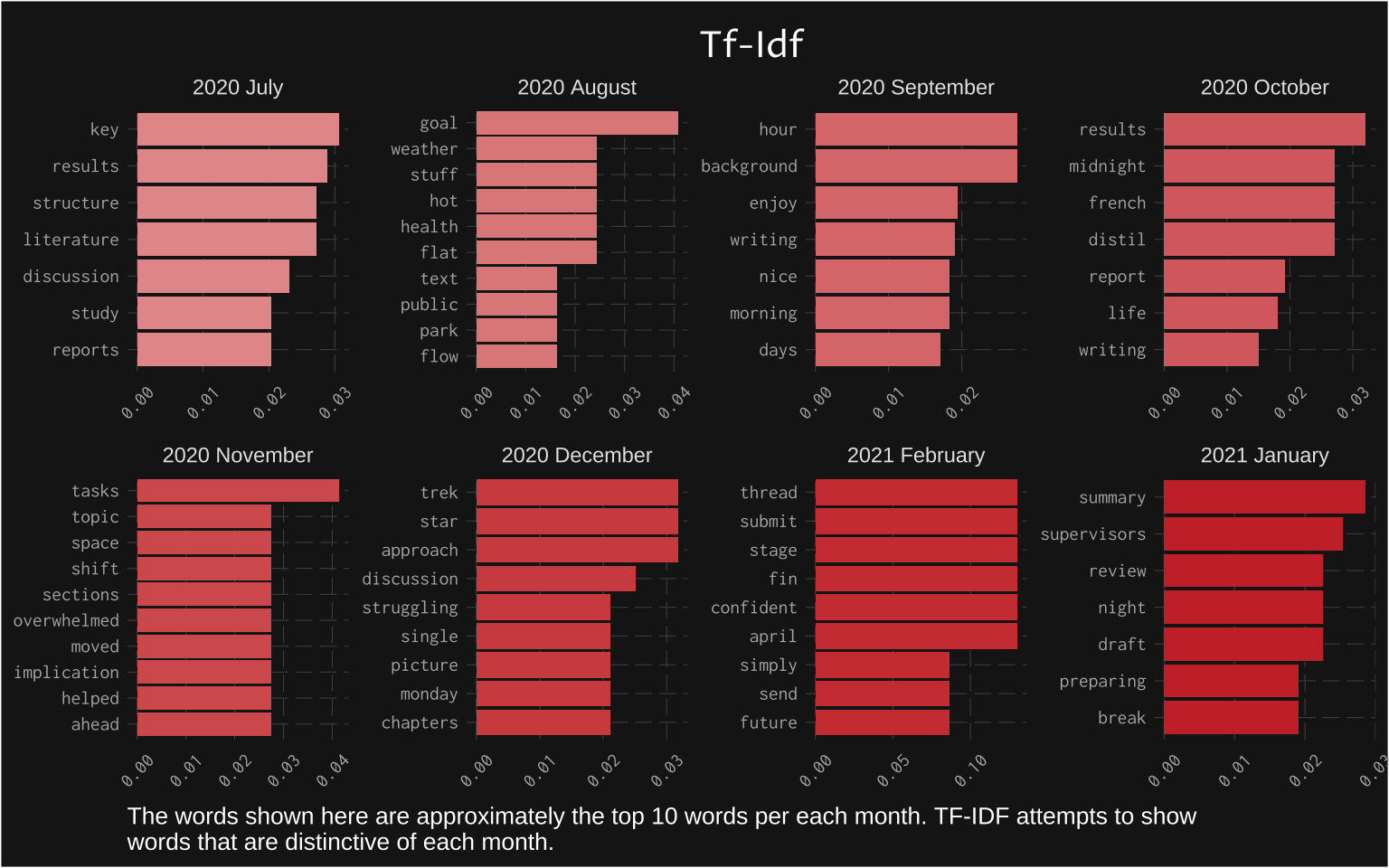
The problem with simple frequencies is that they do not account for features of text that are unique and important. A simple approach to use is either rank and weight frequencies or produce something known as TF-IDF. This measure (in theory) takes into account the total proportion of the word and inverse document term proportion. The document can be anything that further groups the tokens. In this case, my “documents” were months of the challenge.
For example, the word “writing” occurred in August 2020 8 times across 1279 total occurrences; therefore, the TF = 8/1271 = 0.0063. The IDF is log() of the ratio of all documents / documents containing a given word. In this case, “writing” occurred in 6 documents out of 8 (documents = months), hence IDF = log(8/6) = 0.29. Finally, the TF-IDF = 0.29*0.0063 = 0.0018. The formula works in a way that rare words have higher importance (i.e., larger tf-idf means higher importance), and words that are very frequent are weighted down. IDF is, therefore, low for high-occurring words such as stop words.
token_words %>%
     mutate(
          month_date = paste0(year(created_at), " ", months.Date(created_at)),
          month_date = factor(month_date, levels = date_ym_fct,
                              date_ym_fct, ordered = TRUE)) %>%
     count(word, month_date, sort = TRUE) %>%
     mutate(
          total = sum(n),
          word = reorder(word, n),
          proportion = n / sum(n)) %>%
     bind_tf_idf(word, month_date, n) %>%
     arrange(desc(tf_idf))
- Sentiment analysis is really just an extension of a dictionary approach. The idea is to associate each word with a certain category of sentiment, for example, “good” will be categorized as positive. The way it works in tidytext is that each word is
inner_jointo a group in the sentiment dictionary. It can then be counted how many positive words occurred or what was the ratio of positive / negative.
- Sentiment analysis is really just an extension of a dictionary approach. The idea is to associate each word with a certain category of sentiment, for example, “good” will be categorized as positive. The way it works in tidytext is that each word is
bing <- get_sentiments("bing")

sentiment_token_overall <-  token_words %>%
        inner_join(bing) %>%
        count(word, sentiment, sort = TRUE) %>%
        mutate(
             rownumber = row_number(),
             total = sum(n),
             word = reorder(word, n),
             proportion = n / sum(n))
Presenting Text Analysis using ggplot2#
The last section will present the text analyzing of the corpus. I aim to deliver these results by presenting less text and more visuals; therefore, I will comment scarcely. If you want to see how each visual was produced, please see the following code.
I will present the distribution of tokens, frequencies, TF-IDF, and conclude with sentiment analysis.
Distribution of Tokens#
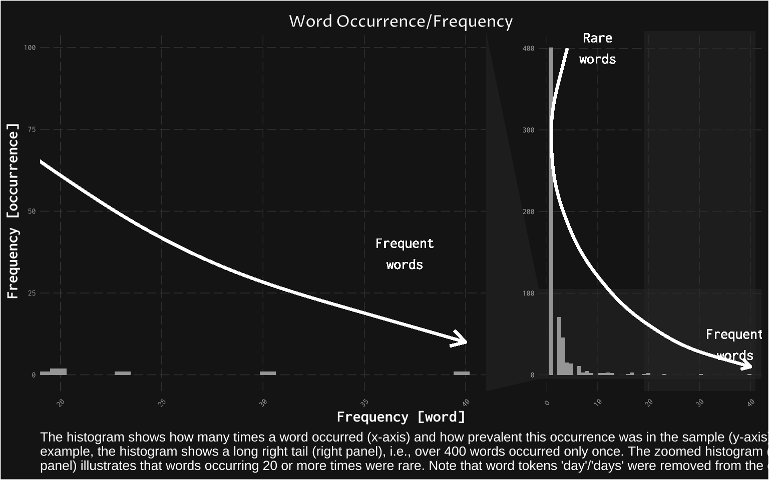
The first thing I look at is a histogram showing a distribution of how many times words occurred in the corpus. The histogram shows that words typically occurred only once, and only on rare occasions occurred more than that. This is fairly typical for the analysis of text (many words occur few times, and few occur many times).
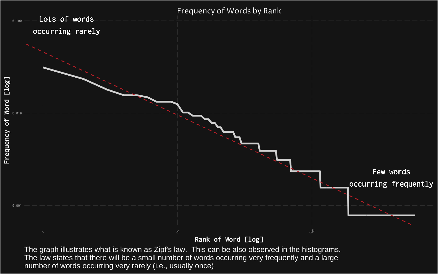
This is often the subject of further research as it is interesting to look at the relationship between word frequency and its rank. Below, I am illustrating this using a classical example known as Zipf’s Law.
Zipf’s law states that the frequency that a word appears is inversely proportional to its rank.
Frequencies of Word and Sentence Tokens#
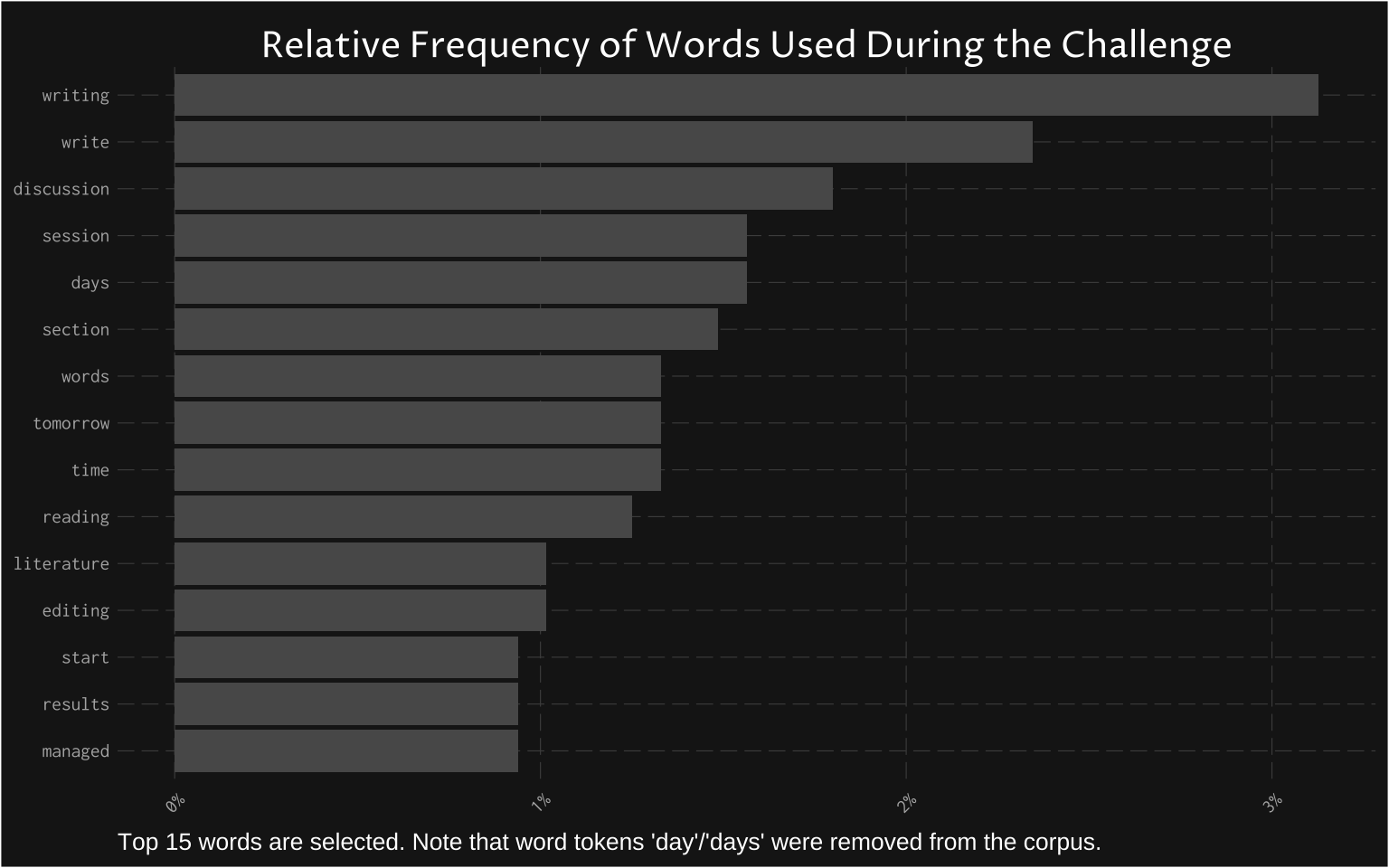
An elegant way to present data from text analysis is to show how many times certain tokens (words or sentences) occurred, what percentage of the corpus did a particular word cover, and illustrate examples of common and rare words.
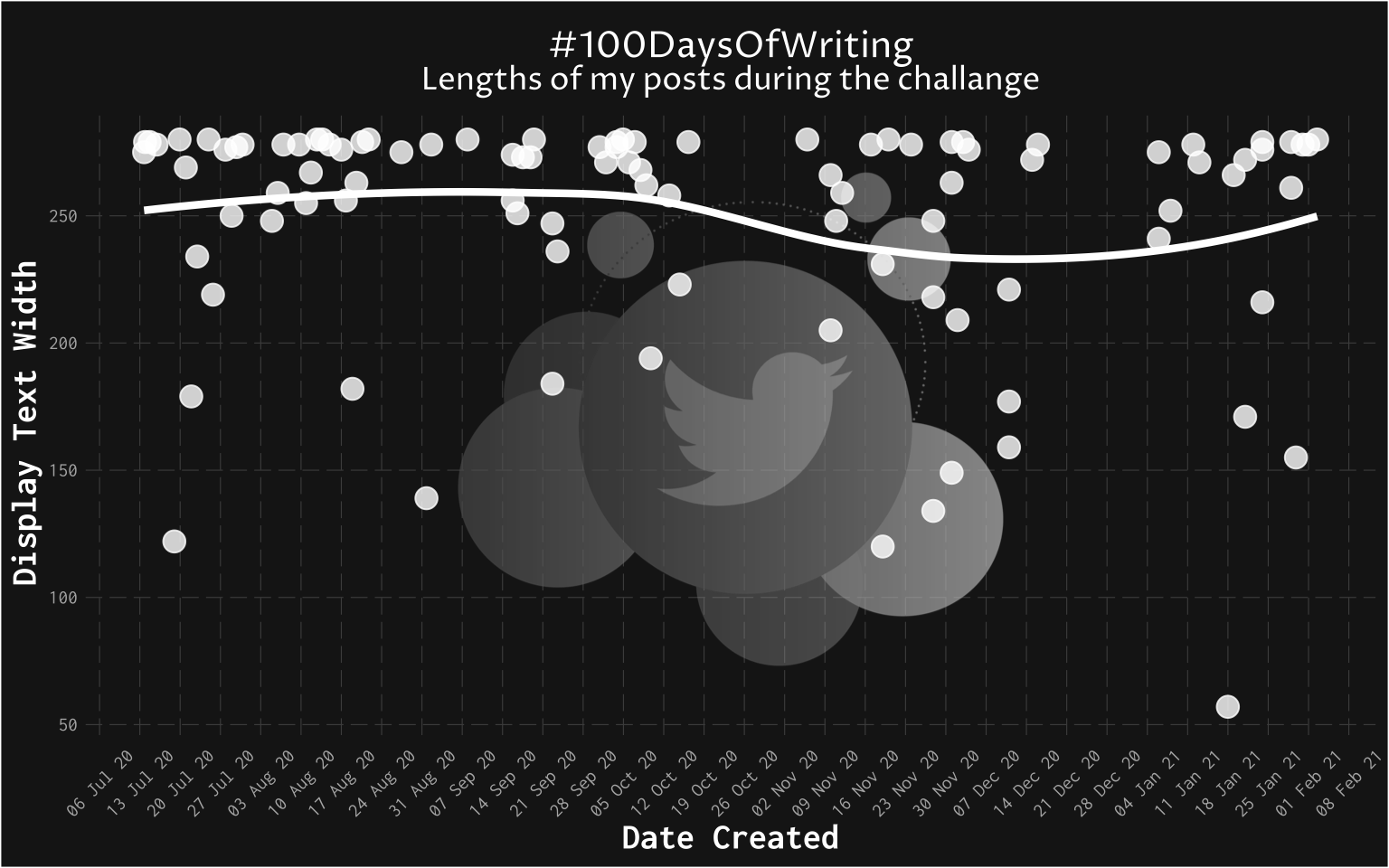
I show below the frequency and relative frequency of word tokens, and a sample of sentences in relationship to their length.
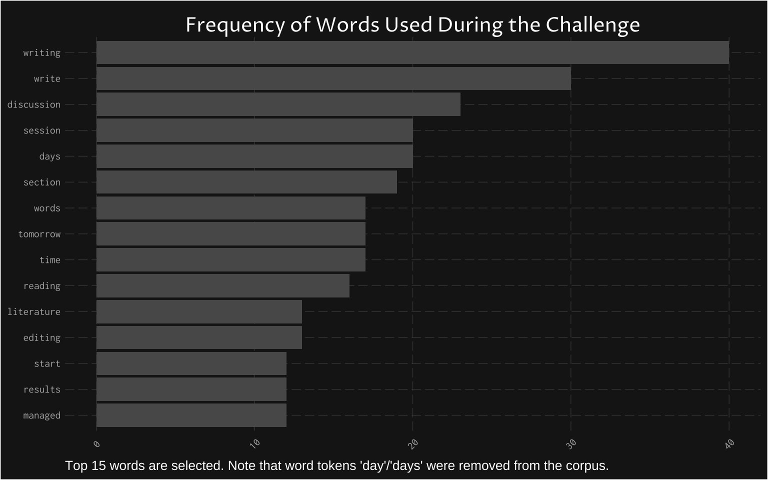
Frequency of common words (top 15) should not be surprising to anyone who knows the corpus. The most common word (after removing some stop words and the “day” word) was “writing”. This is helpful to get a quick sense of what is in the corpus.
Relative frequency then shows the information above as relative to the whole corpus.
Visualizing examples of sentences was a little difficult as I had to find a creative way to present the sentence. I chose using only a sample of sentences and present them as an association with their length. The lengths of sentences were binned, and these bins were then used to sample.

The above can also be shown as a tabular output. Which might be a little more user-friendly.
Display Width | Sentences | Date |
|---|---|---|
57 | [[character]] | 2021-01-17 |
122 | [[character]] | 2020-07-18 |
134 | [[character]] | 2020-11-27 |
139 | [[character]] | 2020-08-31 |
149 | [[character]] | 2020-12-01 |
159 | [[character]] | 2020-12-10 |
177 | [[character]] | 2020-12-10 |
182 | [[character]] | 2020-08-18 |
194 | [[character]] | 2020-10-09 |
205 | [[character]] | 2020-11-09 |
218 | [[character]] | 2020-11-27 |
234 | [[character]] | 2020-07-22 |
241 | [[character]] | 2021-01-05 |
256 | [[character]] | 2020-08-17 |
263 | [[character]] | 2020-12-01 |
276 | [[character]] | 2020-07-27 |
TF-IDF#
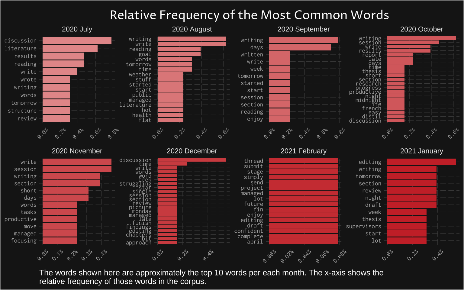
I covered what TF-IDF is above. Here I am presenting the TF-IDF in the context of months. First, I show the relative frequency (%) of words per each month. This simply extends the frequencies by grouping the tokens by month.
This starts to show much more interesting findings. For example, months were not consistently just about writing. As I was nearing the end of the challenge, I was finishing discussion, and eventually, I went onto editing. This is something worth stressing in text analysis. Any natural groupings are, in my opinion, a far better way to interpret results than throwing tokens into a topic modelling or similar classification method. This is because without some prior sense of what data is about, the result of these complicated models is usually impossible to interpret.
TF-IDF then tries to account for words that are important relative to other months. In this context, words such as “writing” are essentially treated as obvious enough to not be worth analysing (the same way an analyst would remove stop words). The result is drastically different bar charts showing some other words that defined my writing experience.
Sentiment#
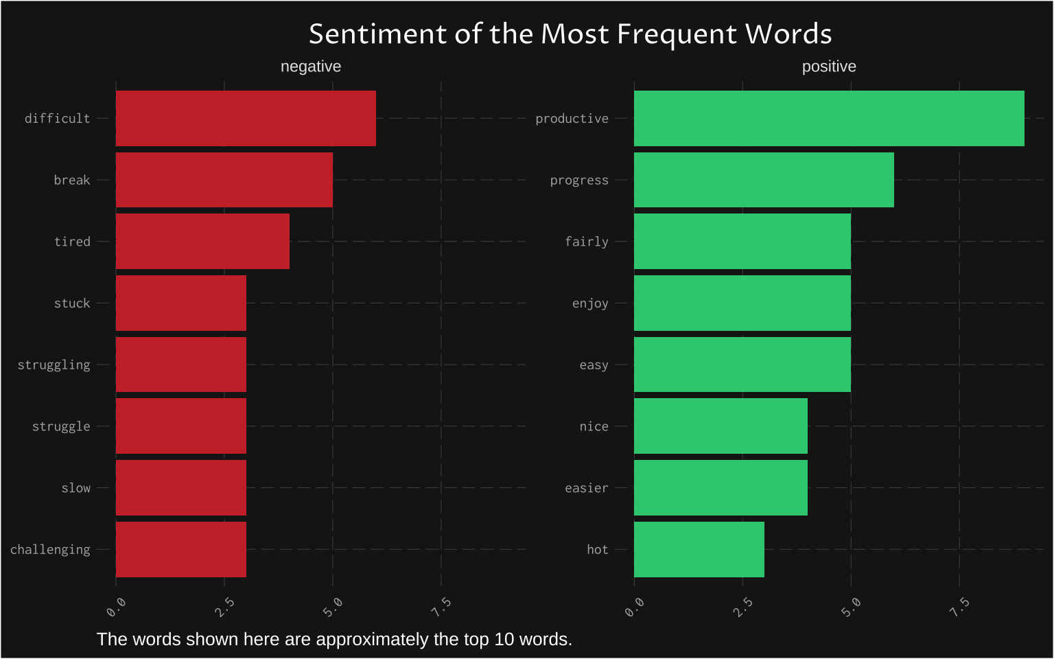
One of the very popular and perhaps overused text analytical methods is sentiment analysis. The idea of sentiment analysis is that it provides a fast and standardized way of associating words with emotions. This is usually done by using a dictionary approach to join defined words to words in the corpus. It is used to evaluate many words and save the analyst’s time but it may not be suitable for all corpora and sometimes it fails in comparison to qualitative methods where the analyst categorises the words on his or her own. The sentiment analysis below will show three charts.
First, I present a relative frequency of the most common negative and positive sentiment. These are interesting words to me as it shows how I felt about the challenge of writing my thesis at times or what was pleasant.
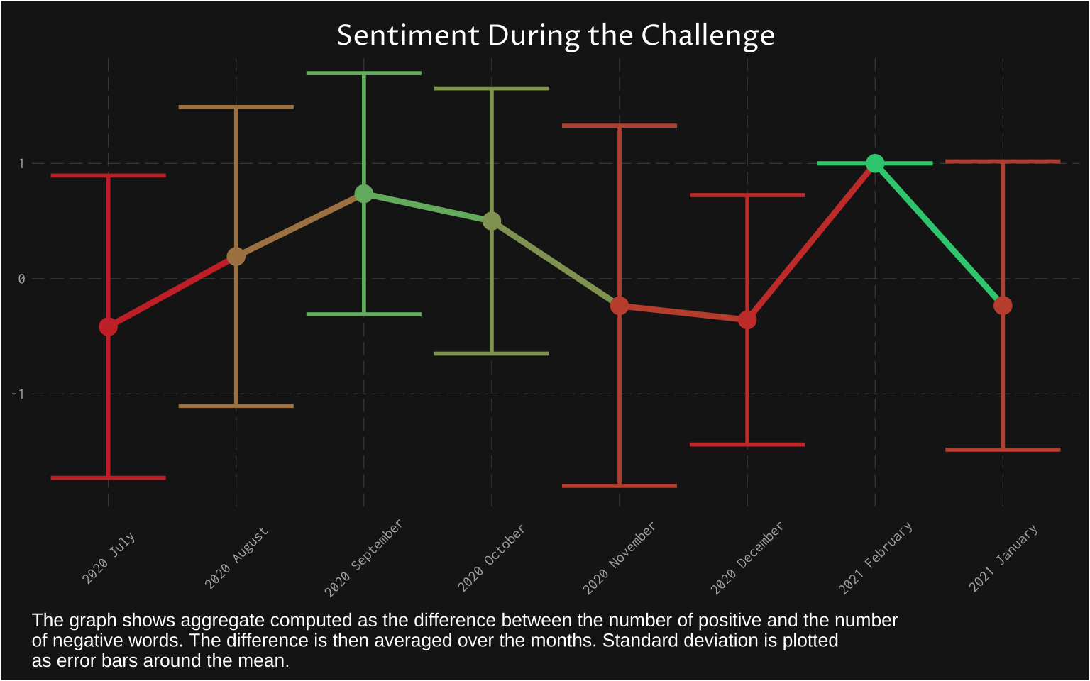
I also felt it was important to provide some idea of how sentiment changed over time. Surprisingly, at the beginning, the sentiment was on average more negative. Maybe I was motivated but realised it is also challenging. This is a very rough idea and you can see that these vary a lot in their “errors” (the bar shows standard deviation around the mean).
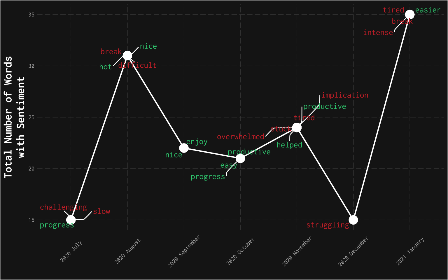
Finally, I tried to show which words were prominent each month. The x-axis dates, y-axis number of words, and around the points are samples of those words. This overlaps with the previous graphs in terms of the middle part of the challenge containing the most positive sentiment.
Conclusion#
This concludes the text analysis and my writing challenge. It was interesting for me to see the challenge presented like this, and I hope potential readers may find this post useful. Please contact me if you have any feedback.