Introduction#
In this post, I’ll share the approach I use to find missing data patterns within text-exclusive datasets. The idea for this post occurred when I was cleaning a messy dataset where participants provided open-ended responses to several questions; these responses were exclusively words. After cleaning the data with the stringr package and labeling missing responses as “NA,” I found it interesting to explore any missing patterns within the data. I searched briefly, but could not find examples that would get me started regarding this type of data; hence, I created this example.
The data I am going to use here is a simple example I’ve created, but it can be generalized to more complex data. I am using several packages here. Some of the mentioned packages are part of the tidyverse, which is a set of packages sharing an underlying philosophy of the so-called tidy data. You can use the whole tidyverse (it’s a lot of packages), but you’ll be fine with using only the dplyr package from the tidyverse. For identification of missing data patterns, I am using VIM and mice packages. I encourage you to read a bit about these amazing packages.
Load required Libraries#
I start by loading the packages. If I would fancy creating a reproducible script that is possible to keep as the data update, check out the package called checkpoint.
library(dplyr)
library(VIM)
library(mice)
Creating random dataset#
My simple data consists of 5 columns and 360 rows. The data are answers about profession provided by participants. Normally, there would be some typos, but that would not be an issue using my approach. The columns are labeled from A to E and represent different conditions.
set.seed(123)
medical_professions <- c("dietitian", "psychologist", NA, "nurse",
                        "pharmacists", "dentist", "surgeon")

df <- as_tibble(replicate(5, sample(medical_professions, 360,
rep = TRUE)), .name_repair = "unique")

names(df) <- c("A", "B", "C", "D", "E")
Overview of my data#
Let’s overview my simple data first.
head(df)
# A tibble: 6 × 5
  A            B            C           D           E
  <chr>        <chr>        <chr>       <chr>       <chr>
1 surgeon      dentist      <NA>        nurse       surgeon
2 surgeon      surgeon      nurse       pharmacists nurse
3 <NA>         dentist      pharmacists <NA>        dentist
4 dentist      dietitian    dentist     dietitian   surgeon
5 <NA>         nurse        pharmacists <NA>        nurse
6 psychologist psychologist dentist     <NA>        surgeon

tail(df)
# A tibble: 6 × 5
  A           B            C            D            E
  <chr>       <chr>        <chr>        <chr>        <chr>
1 surgeon     dentist      psychologist surgeon      pharmacists
2 surgeon     surgeon      nurse        nurse        pharmacists
3 <NA>        nurse        dietitian    dentist      pharmacists
4 dietitian   psychologist dietitian    <NA>         dentist
5 pharmacists dietitian    dentist      <NA>         psychologist
6 surgeon     pharmacists  psychologist psychologist dentist

dim(df) # 360 x 5 columns
[1] 360   5

sum(is.na(df)) # 265 missing values
[1] 257

mean(is.na(df)) # 15% missing percent
[1] 0.1427778

mean(!complete.cases(df)) # 53% rows contain at least one missing value
[1] 0.5277778
VIM Package to show patterns#
Assuming my missing data are labeled as NA, I can use a great visualization function aggr from VIM package. I will disable the proportions output by specifying prop = FALSE and allow representation of missing values using numbers by indicating numbers = TRUE.
library(VIM)
aggr(df, prop = FALSE, numbers = TRUE)
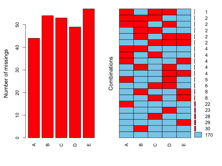
The resulting graph shows the number of missing values on the left and the pattern of missing values on the right; luckily, the most common pattern is that all columns are non-missing. However, a lot of responses in conditions “B” and “A” seemed to be missing. For example, I may have changed the instructions in those conditions or the sample of participants from conditions “B” and “A” thought my experiment is particularly boring.
Either way, I can go even a step further and visualize the missing pattern of individual rows with something called a shadow matrix.
Shadow matrix#
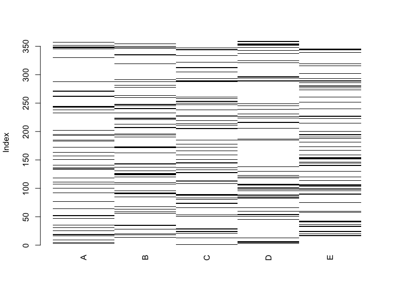
To use the shadow matrix (e.g.: R in Action, page 360) means transforming our data into a set of logical values. If there is a missing value, I will assign TRUE; if the value is non-missing, I will assign FALSE. In numerical terms, this procedure replaces all values that are missing with 1 and values that are non-missing with 0.
Now I can use the function matrixplot from VIM package. All 1 that are missing are represented with a black line.
library(VIM)
shadowmatrix <- as_tibble(abs(is.na(df)))
matrixplot(shadowmatrix)
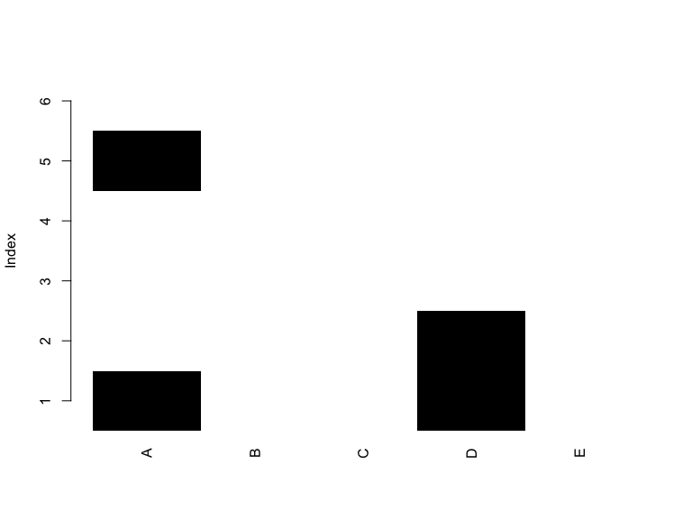
I could also visualize specific rows only. For example, rows 5 to 10.
matrixplot(shadowmatrix[5:10,])
Displaying the pattern again#
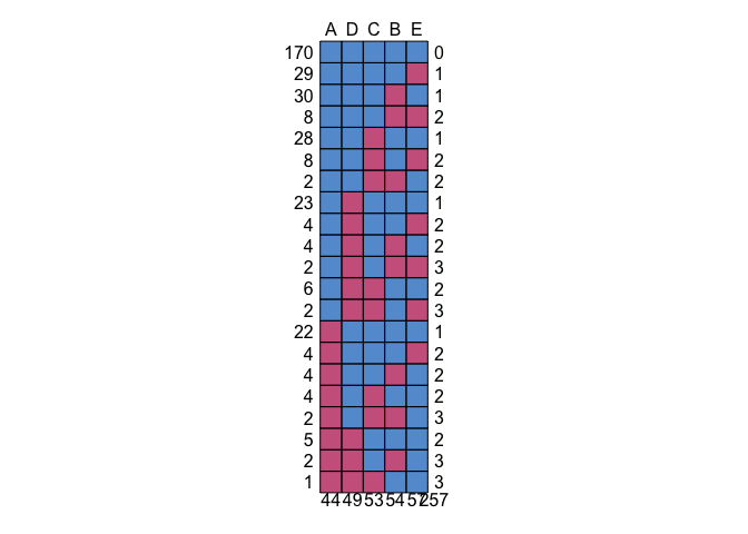
While visualizing individual rows, as mentioned above, is possible, it might be better to use another function, in particular, md.pattern function from the mice package.
This function would not work on the original data that contained strings, but since I have transformed it into a shadow matrix, it will work.
First of all, the function focuses on showing NA patterns; however, those are labeled as number 1, therefore I need to transfer them to NA.
shadowmatrix.NA <- shadowmatrix
Replace all 1 with NA#
The safest way to replace any value as NA is to use is.na function from base R.
is.na(shadowmatrix.NA) <- shadowmatrix.NA == 1
Now I have the shadow matrix with NA labels; let’s use the md.pattern function.
missing.pattern <- tibble(md.pattern(shadowmatrix.NA))
head(missing.pattern) # Top rows
# A tibble: 6 × 1
  `md.pattern(shadowmatrix.NA)`[,"A"] [,"D"] [,"C"] [,"B"] [,"E"] [,""]
                                <dbl>  <dbl>  <dbl>  <dbl>  <dbl> <dbl>
1                                   1      1      1      1      1     0
2                                   1      1      1      1      0     1
3                                   1      1      1      0      1     1
4                                   1      1      1      0      0     2
5                                   1      1      0      1      1     1
6                                   1      1      0      1      0     2

tail(missing.pattern) # Bottom rows
# A tibble: 6 × 1
  `md.pattern(shadowmatrix.NA)`[,"A"] [,"D"] [,"C"] [,"B"] [,"E"] [,""]
                                <dbl>  <dbl>  <dbl>  <dbl>  <dbl> <dbl>
1                                   0      1      0      1      1     2
2                                   0      1      0      0      1     3
3                                   0      0      1      1      1     2
4                                   0      0      1      0      1     3
5                                   0      0      0      1      1     3
6                                  44     49     53     54     57   257
The unlabeled column indicates the number of missing cases in each missing data pattern. Not surprisingly, the first row has no missing cases. The last row indicates a summary of missing values in each condition (compare it to the visualization created above with aggr function). Finally, the total number of missing values is showed at the bottom of the unlabeled column; it should be the same number as the one from sum(is.na(df)) output.
Identify missing values#
Finally, I might decide that rows with 3 or more missing values across all conditions are too much. To see which rows are having 3 or more missing values across all conditions, I can use the command below.
which(apply(shadowmatrix, 1, sum) >= 3)
[1]  96 107 120 172 185 226 288 289 348
Thank you for reading! See you next time.
Reproducibility disclaimer#
Please note that this is an older post. While I can guarantee that the code below will work at the time the post was published, R packages are updated regularly and it is possible that the code will not work in the future. Please see below the R.version to see the last time the code was checked.
R.version
platform       aarch64-apple-darwin20
arch           aarch64
os             darwin20
system         aarch64, darwin20
status
major          4
minor          3.2
year           2023
month          10
day            31
svn rev        85441
language       R
version.string R version 4.3.2 (2023-10-31)
nickname       Eye Holes